Introduction to Federated Machine Learning with Example

While building your own models with machine learning, whether you’re constructing image classifiers, recommendation engines, or talkative GPT models, you may quickly encounter common issues. These include the lack of data for learning, or conversely, a shortage of computing power when dealing with a surplus of data, as well as privacy concerns and insufficient system elasticity to scale your learning progress.
With the increasing interest in the use of mobile and IoT devices, a vast amount of data can be found on end-users’ devices or within private companies’ storage. They could serve as excellent sources for training your model. However, unfortunately, in manny cases you cannot just copy this data and store it in your own storage for learning purposes. But what if I were to tell you that there is a way to train a model even when you cannot transfer the data to your disks? This is where federated machine learning comes in.
What is Federated Machine Learning?
But what is federated machine learning even at the first place? Well, in the vast land of the internet, we may find a few interesting definitions.
Federated learning (also known as collaborative learning) is a sub-field of machine learning focusing on settings in which multiple entities (often referred to as clients) collaboratively train a model while ensuring that their data remains decentralized. [1]
In federated optimization, the devices are used as compute nodes performing computation on their local data in order to update a global model. (…) Additionally, since different users generate data with different patterns, it is reasonable to assume that no device has a representative sample of the overall distribution. [2]
Federated learning is a way to train AI models without anyone seeing or touching your data, offering a way to unlock information to feed new AI applications. [3]
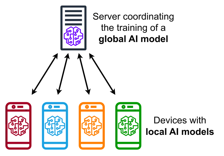
For me, these three quotations above can clearly describe what federated learning is about. You can see that according to these definitions, the learning process is no longer taking place on one centralized device. Instead, each client is participating in training its own version of the global model, which is then merged together with other partial models from other clients again into one global model.
At this point, you may be wondering, if all of the clients train their own local models, how is the one final model achieved? Actually, there are a few methods to amalgamate all the local models into one, but in most cases, at the beginning, you will probably deal with the one called federated averaging.
In this approach, the server sends weights (also referred to as parameters later) to a group of selected clients. Weights may be a result of the model pre-trained on the small batch of data you own or can be completely random at the starting point as well. Then clients receive these weights and rebuild the local model with them, then perform a short set of training with the data it has and return new weights from the result of training to the server. When the server receives all the new weights, it uses a weighted average to create new global weights. Then the new weights are sent to all clients, and the whole process repeats a few times before the final model is built.
Now that we have a high-level understanding of how things are working here, we may proceed to building some example knowledge. To make our lives simpler, we won’t handle everything ourselves but instead, we will use one of the available frameworks for federated machine learning, which is Flower AI.
What is Flower AI?
Flower AI describes itself as a unified approach to federated learning, analytics, and evaluation, which federates any workload, allowing you to use any machine learning framework and any programming language you wish. No matter if you prefer PyTorch, TensorFlow, JAX, or fastai, you are free to go with any of them. It does this while addressing major concerns like data privacy, geographical data distribution, and using devices with limited computing power like smartphones or IoT devices.
It is flexible, scalable, and ensures not to compromise private data. Flower AI comes with a bunch of quick starter projects and detailed documentation covering many use cases. You can find more about it on their website at flower.ai.
What will we build?
For the sake of this article, we will build a pretty “hello world” example of a machine learning application — an image classifier, particularly a handwritten letters classifier. Here, we will have three clients, each of them having about 250 samples spread among ten data classes (letters from “A” to “J”). As a machine learning framework, we will use TensorFlow together with Flower AI to federate the learning process. Even though in this example, the server and client applications will be started locally, it can also be done via a network.
If you want to build the example project while following this article, you will have to install the following packages:
1
pip install flwr tensorflow matplotlib scikit-learn
Alternatively, you may use the requirements.txt file provided with the whole code in my GitHub repository.
Building model
If you already have some experience working with TensorFlow, there won’t be anything difficult for you in this section. We will start by building a pretty common convolutional network, often used for image classification.
1
2
3
4
5
6
7
8
9
10
11
12
13
def get_model() -> keras.Model:
    model = keras.Sequential([
        keras.layers.Input(shape=(100, 100, 1)),
        keras.layers.Conv2D(8, 5, activation='relu', kernel_initializer='variance_scaling'),
        keras.layers.MaxPooling2D(strides=(2, 2)),
        keras.layers.Conv2D(16, 3, activation='relu', kernel_initializer='variance_scaling'),
        keras.layers.Flatten(),
        keras.layers.Dense(units=10, activation='softmax', kernel_initializer='variance_scaling')
    ])

    model.compile(optimizer='adam', loss='sparse_categorical_crossentropy', metrics=['accuracy'])

    return model
This may not be the most advanced convolutional network you’ve seen, but for demonstration purposes, this will work quite well. So let’s stick with this.
Server-side application
Now we need a server that will orchestrate the learning process. Here’s where Flower AI really comes in. With Flower AI, we may decide about which strategy for learning we will use. Here, we will go with one of the most common federated aggregation strategies, but we will customize it a little bit.
First, after each round of training, I want to have the current accuracy printed out. We may achieve this by extending the aggregate_evaluate method and using metrics received from clients. Second, I want to have our model saved, but not only that, I would also like to have it saved after each round of training. We will achieve this by extending the aggregate_fit method and storing the current version of the model in a location of our choice.
Both of these requirements can be covered with the following code.
1
2
3
4
5
6
7
8
9
10
11
12
13
14
15
16
17
18
19
20
21
22
23
24
class CustomStrategy(fl.server.strategy.FedAvg):
    def aggregate_evaluate(self,  server_round: int, results: List[Tuple[ClientProxy, EvaluateRes]], failures: List[Union[Tuple[ClientProxy, EvaluateRes], BaseException]]) -> Tuple[Optional[float], Dict[str, Scalar]]:
        if not results:
            return None, {}

        loss, metrics = super().aggregate_evaluate(server_round, results, failures)
        accuracies = [r.metrics["accuracy"] * r.num_examples for _, r in results]
        examples = [r.num_examples for _, r in results]

        accuracy = sum(accuracies) / sum(examples)
        log(INFO, f"Round {server_round} accuracy aggregated from {len(results)} clients: {accuracy}")

        return loss, {"accuracy": accuracy}

    def aggregate_fit(self, server_round: int, results: List[Tuple[ClientProxy, FitRes]], failures: List[Union[Tuple[ClientProxy, FitRes], BaseException]]) -> Tuple[Optional[Parameters], Dict[str, Scalar]]:
        parameters, metrics = super().aggregate_fit(server_round, results, failures)

        if parameters is not None:
            model = get_model()
            model.set_weights(fl.common.parameters_to_ndarrays(parameters))
            model.save(f"models/model-round-{server_round}.keras")
            log(INFO, f"Saving round {server_round} model")

        return parameters, metrics
When we have this ready, we may prepare our server by defining the server address and how many rounds of training should take place. We will provide these details with command arguments when starting our script later.
1
2
3
4
5
6
7
8
9
10
11
12
13
14
15
def main(server_address: str, num_rounds: int) -> None:
    fl.server.start_server(
        server_address=server_address,
        config=fl.server.ServerConfig(num_rounds=num_rounds),
        strategy=CustomStrategy(min_available_clients=3, min_fit_clients=3, min_evaluate_clients=3),
    )


if __name__ == "__main__":
    parser = argparse.ArgumentParser(description='Server')
    parser.add_argument('--server-address', type=str, required=True)
    parser.add_argument('--num-rounds', type=int, required=True)
    args = parser.parse_args()

    main(server_address=args.server_address, num_rounds=args.num_rounds)
To have a more detailed overview of the training process, I would like to have a visualized graph of accuracy and loss changes. The start_server method returns a history object which we may use to draw the chart of our model’s learning progress.
1
2
3
4
5
6
7
8
9
10
11
12
13
14
15
16
17
18
19
20
21
def plot(history: fl.server.history.History) -> None:
    accuracy = history.metrics_distributed["accuracy"]
    accuracy_index = [data[0] for data in accuracy]
    accuracy_value = [100.0 * data[1] for data in accuracy]

    loss = history.losses_distributed
    loss_index = [data[0] for data in loss]
    loss_value = [data[1] for data in loss]

    plt.plot(accuracy_index, accuracy_value, "r-", label="Accuracy")
    plt.plot(loss_index, loss_value, "b-", label="Loss")
    plt.grid()
    plt.xlabel("Round")
    plt.ylabel("Accuracy (%)")
    plt.title("Handwritten Letters Classifier - Federated Accuracy")
    plt.show()


def main(server_address: str, num_rounds: int) -> None:
    history = fl.server.start_server(...)
    plot(history)
Client-side application
When the server side is ready, we need to build the client application as well. Here we can simply start by extending NumPyClient from Flower AI and implement the get_parameters, fit, and evaluate methods to make it work.
The get_parameters, as its name suggests, returns the parameters (weights) from the current version of the model. The fit method is used to train the model and returns the tuple compounded of weights after training, the size of the dataset used for training (needed for averaging weights on the server side), and the metrics we are interested in. The evaluate method, as its name suggests, checks the progress of our model and is expected to return loss, the size of the validation dataset, and metrics we want to pass to the server.
1
2
3
4
5
6
7
8
9
10
11
12
13
14
15
16
17
18
class Client(fl.client.NumPyClient):
    def __init__(self, model: keras.Model, trainset: tf.data.Dataset, validset: tf.data.Dataset):
        self.model = model
        self.trainset = trainset
        self.validset = validset

    def get_parameters(self, config: Dict[str, Scalar]) -> NDArrays:
        return self.model.get_weights()

    def fit(self, parameters: NDArrays, config: Dict[str, Scalar]) -> Tuple[NDArrays, int, Dict[str, Scalar]]:
        self.model.set_weights(parameters)
        self.model.fit(self.trainset, epochs=1, batch_size=32)
        return self.model.get_weights(), len(self.trainset), {}

    def evaluate(self, parameters: NDArrays, config: Dict[str, Scalar]) -> Tuple[float, int, Dict[str, Scalar]]:
        self.model.set_weights(parameters)
        loss, accuracy = self.model.evaluate(self.validset)
        return loss, len(self.validset), {"accuracy": accuracy}
The next step will be to load data for training, and here we will simply use image_dataset_from_directory from Keras utils, which allows loading the data split into training and validation datasets. Our images are 100x100px each, and black and white, so we will use them in grayscale to not bother about unnecessary color channels.
1
2
3
4
5
6
7
8
9
10
11
12
def get_datasets(data_dir: str) -> tf.data.Dataset:
    datasets = keras.utils.image_dataset_from_directory(
        directory=data_dir,
        validation_split=0.1,
        subset="both",
        color_mode="grayscale",
        image_size=(100, 100),
        shuffle=True,
        batch_size=32,
        seed=522437,
    )
    return datasets
When we can load the data, we may start the client, which requires the address of the server where it should connect and the path to the data, which in this example is stored in one of the subdirectories on the local disk.
1
2
3
4
5
6
7
8
9
10
11
12
13
14
15
16
17
def main(server_address: str, data_dir: str) -> None:
    trainset, validset = get_datasets(data_dir)
    model = get_model()

    fl.client.start_numpy_client(
        server_address=server_address,
        client=Client(model, trainset, validset)
    )


if __name__ == "__main__":
    parser = argparse.ArgumentParser(description='Client')
    parser.add_argument('--server-address', type=str, required=True)
    parser.add_argument('--data-dir', type=str, required=True)
    args = parser.parse_args()

    main(server_address=args.server_address, data_dir=args.data_dir)
Let’s start training
Perfect! When both applications are ready, we may start them in separate sessions of the terminal. Our setup requires one server and three clients, and the server has to be started first.
1
2
3
4
python server.py --server-address=0.0.0.0:8080 --num-rounds=6
python client.py --server-address=127.0.0.1:8080 --data-dir=./data/client-1
python client.py --server-address=127.0.0.1:8080 --data-dir=./data/client-2
python client.py --server-address=127.0.0.1:8080 --data-dir=./data/client-3
As a result, you will see the pretty verbose output of the training process with information about learning progress, successful and failed sessions, accuracy, and loss metrics. At the end, the chart of progress will appear on your screen. The red line presents accuracy, and the blue line presents loss in each learning round.

Additionally, with the strategy we prepared, our model will be saved in the models directory. We may use them to check it out on some of the handwritten letters. With the script presented below, we can load the model and use it to predict the letter on the given image.
1
2
3
4
5
6
7
8
9
10
11
12
13
14
15
16
17
18
19
20
21
22
23
24
25
26
class_names = ['a', 'b', 'c', 'd', 'e', 'f', 'g', 'h', 'i', 'j']


def main(model_path: str, image_path: str) -> None:
    model = keras.models.load_model(model_path)

    image = keras.utils.load_img(image_path, target_size=(100, 100), color_mode="grayscale")
    image = keras.utils.img_to_array(image)
    image = tf.expand_dims(image, 0)

    prediction = model.predict(image)
    score = tf.nn.softmax(prediction[0])

    print(
        "This image most likely belongs to {} with a {:.2f} percent confidence."
        .format(class_names[np.argmax(score)], 100 * np.max(score))
    )


if __name__ == "__main__":
    parser = argparse.ArgumentParser(description='Validator')
    parser.add_argument('--model-path', type=str, required=True)
    parser.add_argument('--image-path', type=str, required=True)
    args = parser.parse_args()

    main(args.model_path, args.image_path)
You can run this with the following command:
1
python predict.py --image-path=./data/client-2/g/1691660116597.png --model-path=./models/model-round-6.keras
And then you will see the output: This image most likely belongs to 'g' with a 23.20 percent confidence. It doesn’t seem to be too confident about that, but it guessed the letter correctly after all.
The last thing I would like to have here is the confusion matrix for a preview, which we may achieve with the following code.
1
2
3
4
5
6
7
8
9
10
11
12
13
14
15
16
17
18
19
20
21
22
23
24
25
26
27
28
29
30
31
32
33
34
35
36
37
38
39
40
class_names = ['a', 'b', 'c', 'd', 'e', 'f', 'g', 'h', 'i', 'j']


def get_test_data(data_dir: str) -> Tuple[np.ndarray, np.ndarray]:
    dataset = keras.utils.image_dataset_from_directory(
        directory=data_dir,
        color_mode="grayscale",
        image_size=(100, 100),
        shuffle=True,
        batch_size=32,
        seed=522437,
    )
    test_images, test_labels = zip(*dataset.unbatch().as_numpy_iterator())
    test_images = np.array(test_images)
    test_labels = np.array(test_labels)

    return test_images, test_labels


def main(model_path: str, data_dir: str) -> None:
    model = keras.models.load_model(model_path)
    test_images, test_labels = get_test_data(data_dir)

    predictions = model.predict(test_images)
    predicted_labels = np.argmax(predictions, axis=1)

    matrix = confusion_matrix(test_labels, predicted_labels, labels=range(10))
    display = ConfusionMatrixDisplay(confusion_matrix=matrix, display_labels=[s[-1] for s in class_names])
    display.plot(cmap=plt.cm.Blues, values_format='.4g')

    plt.show()


if __name__ == "__main__":
    parser = argparse.ArgumentParser(description='Validator')
    parser.add_argument('--model-path', type=str, required=True)
    parser.add_argument('--data-dir', type=str, required=True)
    args = parser.parse_args()

    main(args.model_path, args.data_dir)
You can run it and see the output with the command presented below.
1
python confusion.py --model-path=./models/model-round-6.keras --data-dir=./data/client-2
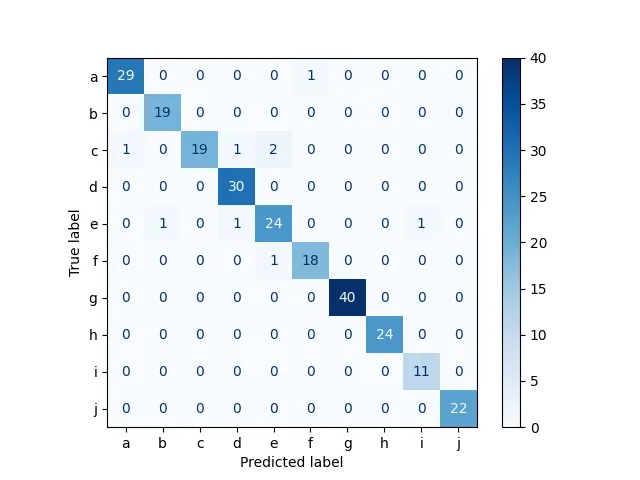
I know that it is not really representative as it was calculated on the same data as used for training, but I will just pass over it for the sake of demonstration :)
Summary
Even though federated learning may seem a bit more complicated than the centralized counterpart, it can bring valuable benefits and solve problems that may be hard to solve with standard approach. I hope that after reading this article, you will find federated machine learning as interesting as I do. Maybe you can already see the application for it in some of your projects, or perhaps you’re considering diving deeper into it. Have fun then.
If you need the whole code from this article in one place, you can find it in my GitHub repository.
Thank you for reading this article. I would love to read your thoughts about federated learning. Maybe you have some experience with it already, or you are considering adopting it for your needs. No matter your position on it, don’t hesitate to share in the comments section.
Don’t forget to check out my other articles for more tips and insights. Happy hacking!
References
¹ Wikipedia, Federated learning
² Jakub Konečný, H. Brendan McMahan, Daniel Ramage, Peter Richtárik. Federated Optimization: Distributed Machine Learning for On-Device Intelligence
³ IBM Blog. What is federated learning?